
Prepare for Parametric Functions
An Exploration of Trigonometry Parametric Functions
by
Sarah Major
This write-up is based on a prompt from Exploration 10, which states:
1. Graph
![]()
How would you change the equations to explore other graphs?
First, we will graph the parametric equations exactly as stated to see what this graph looks like (all images created using Graphing Calculator software):

This produced the graph of the unit circle. If we extend the interval of t, we will obtain the same graph because the points simply complete multiple revolutions around the circle as t increases. We know this from simple trigonometry.
What if we were to add a coefficient of a to cos(t), where a > 1? How would the graph of this function change just within the 2pi interval of t? In Graphing Calculator, we can produce a slider so that we can change the value of a at will. First, we will look at only positive values for a.

We can see that the graph looks like an ellipse. This is because by adding a positive coefficient in front of cos(t), we are multiplying our x-values by this coefficient, increasing them by a factor of a. To connect this back to simple algebra, we are essentially creating a "horizontal stretch". When explaining this to a student who does not understand the algebraic concept of this translation, we can say that we are taking our unit circle and stretching it to the left and right by a factor of a. This could be demonstrated tangibly for an algebra or trigonometry class using something such as a bungee cord.
Digressions aside, as a increases from 1, the domain of our parametric function increases by a factor of a. For instance, for the unit circle, we have a domain of (-1,1). If we multiply cos(t) by, say, 3, our domain would change to (3,3).

Therefore, we produce the translation (x,y) -> (ax,y). This makes sense because algebraically, we are not changing the y-values at all. Though the domain changes when we translate our parent function in this way, the range remains (-1,1) for both parametric equations:

What if we instead multiply sin(t) by a positive value of a? Instead of increasing the x-values by a factor of a, we will increase the y-values by a factor of a:

In essence, we produce the translation (x,y) -> (x,ay). Once again, one could demonstrate this with a tangible object to increase student understanding.
What if we multiply both sin(t) and cos(t) by a? This is simply multiplying the whole parametric function by a, so we are simply increasing the whole unit circle by a factor of a.

One could say that we have created an "a" circle instead of a unit circle.
This translation is (x,y) -> (ax,ay), or (x,y) -> a(x,y) (though one may not want to use this type of notation).
We can extend such translations to positive values a and b such that x = asin(t) and y = bcos(t), where a does not equal b, and, for the sake of this particular analysis, a,b > 1. Such a translation would be (x,y) -> (ax,by). In the case where a > b, we would have a graph similar to the one below (in which a = 3, and b = 2):
![]()
In simplest terms, we "combine" the two translations, the "horizontal stretch and vertical stretch", into one ultimate translation.
What happens when 0 < a < 1? Instead of a "stretch", we have a "shrink". For instance, when we have x = 1/2cos(t), we have the following graph:

In terms of the shape of the graph, we still have an ellipse, but it is essentially “opposite” of our first case. For example, when we multiplied our cosine function by a value that was greater than 1, we increased the x-values of our function and made the left and right sides “longer” than the top and bottom of the function. When we multiply the cosine function by a value smaller than 1, we make the left and right sides “shorter” than the top and bottom of the function. This can be demonstrated tangibly by pushing the sides of a bungee cord together instead of stretching them. However, if doing such a demonstration, make sure to make the disinction that the points (0,1) and (0,-1) do not change between translations.
As with the connection above, multiplying the sine function will "shrink" the range of the parametric equation instead of the domain.

What if instead of multiplying the whole trigonometric function by a value, we instead multiply the value of t within the function by a value? We will first examine the case where 0 < t < 2pi. Let’s first do x = cos(at), beginning with a = 0:

When a = 0, we have a vertical line segment at x = 1. This makes sense because cos(0) = 1, and the range can only be between -1 and 1 because this is our range for our unit circle. Different values of t, regardless of how large, will only produce values between -1 and 1. Now, we will slowly increase our a-value to 1/2:

We could think of our previous line segment as a three-dimensional circle that we cannot see because we are in a two-dimenstional plane. When a = 0, we are looking at the side of the circle, so we cannot see the face of it. When we slowly increase the value of a, it is like we are cutting our circle at the point (1,0) at the back end that we cannot see. As we get to a = 1/2, we are taking our severed end of our circle and pulling it to the point (-1,0) to create a sort of spiral. This could be demonstrated tangibly by taking one coil of a slinky and pulling its open end apart.
What happens when we slowly increase a from 1/2 to 1?

We, of course, obtain our unit circle. With our slinky reference, we can say that we are now taking the end of our slinky from the point (-1,0) and bringing it back around to the point (1,0), only this time, we have rotated the face of our circle to face us. So, as a goes from 0 to 1, we can say that we are rotating a circle 90 degrees.
This oscillation between the points (1,0) and (-1,0) continues as a increases:


If the coils of a slinky were infinitely flexible, we could say that we are continuing to rotate our coil in a circle as a increases. As this coil continues to rotate, we create an oscillation that is just like a two-dimensional cosine function, only three-dimensionally, it is rotating in a circle. In other words, if we took an ordinary cosine function:

Decreased its period:

Took the ends of the function, and connected them together to create a circle (if we rotated the function 90 degrees so that the “right” side of the function were facing “forward”), we would create this type of function. An elementary explanation is that we are taking a highly-oscillating cosine function and turning it into a bracelet for the x-axis to wear.

What if we increase the values that t can be to 4pi?

6pi? 1Mpi? The function would continue its oscillation faster and faster, but the x-axis would still have a nifty bracelet to wear (below, t can be up to 60pi):

What if we switched the value of a to the sine function and made y = sin(at)? Let’s begin once again with 0 < t < 2pi, and let’s begin with a = 0:

The graph is hard to see because it lies on the x-axis, but this time, we have a horizontal line segment extending from x = -1 to 1. As a increases we have the same trend as before except that instead of the x-axis wearing the “bracelet”, we are letting the y-axis wear it:


Notice that we are still “splitting” our function at the same point (1,0), but instead of bringing it over to (-1,0), we let it oscillate between the points (1,1) and (1,-1).
We also have the same trend if we increase the value that t can be:
What if we keep the value of a for both the sine and the cosine function? Having the same value for both will make the domain and range of our parametric function be the same, but as a changes, so do the values for the domain and range. As a increases, we make smaller and smaller circles until a reaches 10, where the figure created is completely filled in. In a three-dimensional space, we could think of this figure as a sphere:


This trend goes into reverse as a increases towards 20. At 20, the trend begins from the beginning again. We can see some similar properties between this parametric function and its parent function. Both will produce a set of points that are equidistant from the origin (sort of). I guess in the simplest sense, we can see that the domain and range will be the same for this function and its parent function.
What if we have a parametric function such that x = cos(at) and y = sin(bt)? How will the function behave if we let the values of t range from 0 to 2pi? Unfortunately, this is hard to generalize because it really depends on our values of a and b. Let’s say that we let b be a constant value, say 5, and we slowly increase a starting at 0:

At the start, the graph looks exactly the same as when we didn’t have b. Let’s increase a slowly (this is when a = 1/2):

We see that the oscillation occurs much more rapidly than in our previous case. The period is much smaller for this function. But as far as wrapping around to create our “bracelet” this occurs at the same rate, and the bracelet is complete when a reaches 1:

We have a unique effect that occurs between the time that a = 1 and a = 1/2b. The period actually increases to the point that when we reach a = 1/2b, we have created a sort of bow tie:

In essence, we have two periods of the oscillating function that wrap around to make our circle, but from our two-dimensional perspective, it looks like a bow tie. From another elementary perspective, it would look like a Pringles chip in three dimensions.
We would expect that since there is a special graph that occurs when a is 1/2 the value of b, we would have a special graph when a is 2/3 the value of b, and we would be right (I could not get the value to be exact, but it is close at a = 3.33):

It looks like one period of the trigonometric function that wraps around on itself.
As a comes closer and closer to the value of b, we see that the graph is attempting to become a circle (a = 4.38):

And once a is equal to the value of b, we have our unit circle:

One interesting graph comes when a is approximately 4.75 (in the figure below, a = 4.73):

The graph looks as though we have a have a series of figures that become more and more like a circle. For instance, if we look near the points (1,1) and (-1,-1), we see something similar to the corners of the square.
Say we drew the line y = x on this graph. As we move the point (1,1) down this line towards the origin, we see that we come in contact with ellipses that are split in half by our line. As we continue down our line, the ellipses become more and more circular.
Now, lets increase our a value to around 4.9 (the figure below is 4.93):

We can see that the "ellipses" are still becoming more and more circular as we move down the line y = x, but they are more so than our previous a value. As we reach a = 5, all of these ellipses have now approached the unit circle.
What happens when a > 5, or our b value? We have the reverse effect. Our circle transitions into a series of ellipses that become less and less like circles as a increases. However, instead of having "corners" at (1,1) and (-1,-1), our corners are at (1,-1) and (-1,1). The first figure is a = 5.20, and the next is a = 6.44:


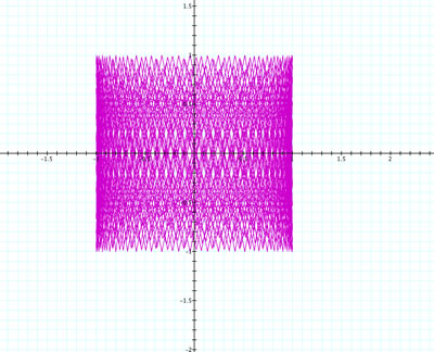
What if we increase the values that t can be? We would meet the same trend from the previous case. Below is when t is extended to 60pi:

We would expect that since a special graph was constructed when a was half the value of b, we would expect a special graph to occur when a is double the amount of b, and we would be right (when t can only go to 2pi):

It looks like all the "peaks" meet at the same point, (1,0).
Why wouldn’t the graph be special when a is 3 times b? Let’s see what happens:

And 4 times?

I’m sensing a pattern when a is a multiple of 2 times b. It seems as though the number of “peaks” is half the ratio of b to a, and the direction that the “peaks” are facing alternates between facing left and right. I predict that when a = 6b, there will be three peaks, and they will face to the right. Below is the graph:

And I would be right! So, if a = 8b, there should be four peaks facing to the left. Here is the graph:

Awesome.